
Simulator Technical Notes
SAI SIMULATOR V1.4 · TECHNICAL NOTES
Technical notes
These notes describe how the SAI (stratospheric aerosol injection) Simulator version 1.4 calculates its results, which data it is trained on, and the limitations of each step. The full code is public in the GitHub repository.
In short: global mean temperature comes from the FaIR simple climate model; regional fields come from linear pattern scaling fitted separately to three Earth system models and averaged with equal weight; the response to SAI is a linear function of the cooling required, fitted to six SAI simulations; latitude-specific and custom injection use an emulator trained on CESM2-WACCM. The Simulator is an emulator of existing simulations, so it inherits their assumptions and cannot represent processes they do not include.
Architecture
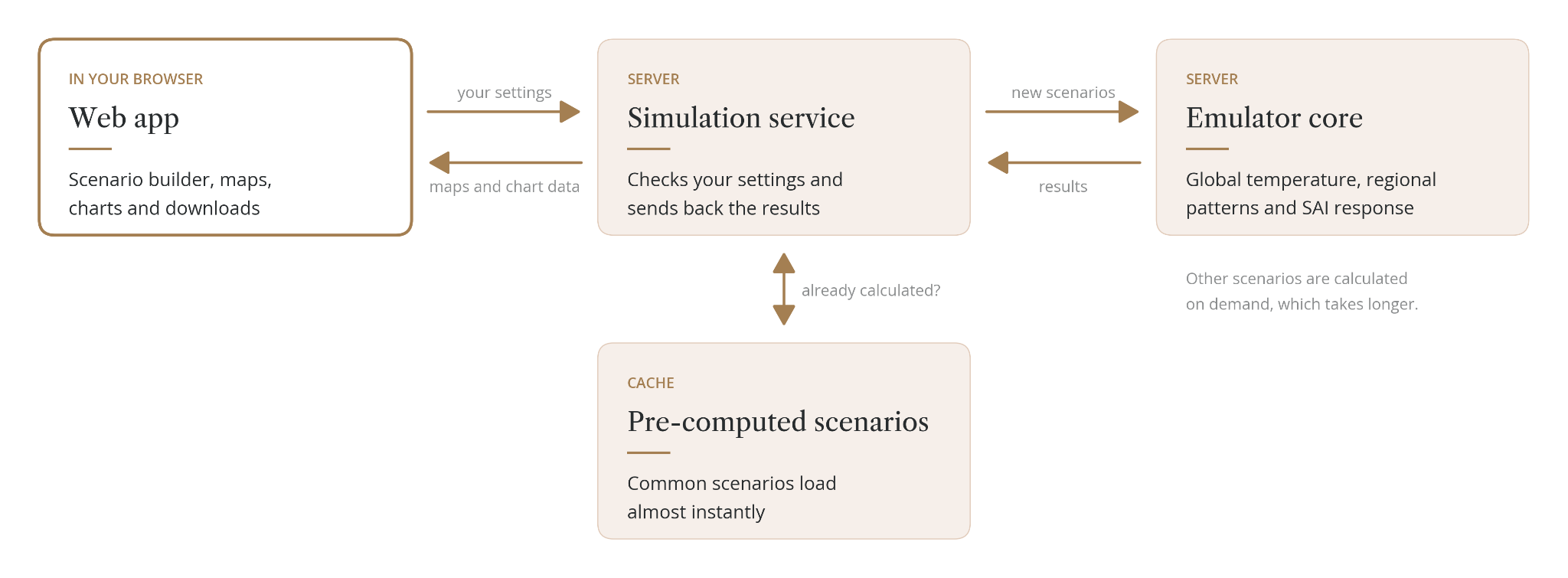
The web app sends your settings to a simulation service, which runs the emulator and returns maps (as GeoTIFF files) and chart data. Common scenarios are pre-computed and returned almost instantly; any other combination is calculated on demand, which takes longer. The simulation service is not a supported public API. To run the Simulator yourself, use the code and instructions in the public repository.
Global mean temperature
- Global mean surface temperature is calculated with FaIR version 2.1.3 (Leach et al., 2021), driven by RCMIP emissions for each SSP, plus solar and volcanic forcing.
- The Simulator runs 100 members of the IPCC AR6-constrained FaIR calibration (calibration v1.2.0), from 1750, and uses the mean of the members. Temperatures are expressed relative to 1850–1900.
- Version 1.4 replaces the CESM-tuned FaIR used in earlier versions.
Limitations. The spread across FaIR members, which reflects uncertainty in climate sensitivity and other parameters, is not carried through to any output.
Regional pattern scaling
- For each climate model and each grid cell, the annual field is regressed linearly on that model's own global mean temperature anomaly (relative to its own 1850–1900 mean).
- The fits use each model's SSP2-4.5 simulation for 2015–2099, with 100 bootstrap replicates that are averaged.
- To produce a projection, the FaIR global temperature is passed through each model's fitted pattern, and the three results are averaged with equal weight. FaIR sets the amount of warming; the models provide the spatial pattern per degree of warming.
- All fields are regridded bilinearly to the CESM2-WACCM grid (0.9375° latitude × 1.25° longitude).
- Projections cover 2015–2100. The historical period (1850–2014) is the multi-model mean of each model's historical ensemble mean.
Limitations. The patterns are trained on SSP2-4.5 only and applied to all eight scenarios, so scenario-specific patterns, for example from different aerosol emissions, are not represented. The relationship is linear in global temperature.
SAI response for the Global strategy
- Each year, the cooling required is the difference between the projected global temperature and the target, or zero where projected warming is already below the target.
- The change in each grid cell is a fixed slope multiplied by the cooling required. SAI ramps up linearly over the first 10 years of deployment.
- The slope is a single least-squares fit through the origin across six SAI simulations. For each, the 2050–2069 mean of the SAI simulation minus the simulation without SAI it branched from is compared with that simulation's global cooling:
- CESM2-WACCM, ARISE simulations targeting 1.5 K, 1.0 K and 0.5 K above pre-industrial (Richter et al., 2022)
- MIROC-ES2H, G6-1.5K and G6-0.5K (Visioni et al., 2026)
- UKESM1-1-LL, G6-1.5K (Visioni et al., 2026)
- Because the fit weights each simulation by the square of its cooling, the models contribute unequally: CESM2-WACCM 51%, MIROC-ES2H 34% and UKESM1-1-LL 15%.
- SO₂ amounts come from latitude-specific slopes (Tg SO₂ per K of cooling) at 30°S, 15°S, 15°N and 30°N, derived from the feedback controller logs of the CESM2-WACCM ARISE simulations for 2050–2069.
Limitations. The response is linear and immediate: after the ramp, global temperature with SAI sits exactly on the target, with no lag or memory. All three models receive the same SAI change, so the SAI response does not vary between models.
Latitude-specific and custom injection
For the Uniform, Temperate zones, Polar, Polar with backup and Northern Hemisphere only locations, and for injection grids edited by hand, the Simulator uses the CIDER emulator (Farley et al., 2026).
- Annual SO₂ injection at each of seven latitudes (60°N, 30°N, 15°N, 0°, 15°S, 30°S, 60°S) is spread evenly over the months of the year.
- SO₂ is converted to aerosol optical depth with a first-order impulse response whose decay speeds up with injection size, so larger injections are less efficient.
- Aerosol optical depth is converted to a climate response with a diffusive response function, multiplied by a response pattern for each latitude derived from CESM2-WACCM.
- This response is added to the multi-model mean projection without SAI. It covers temperature, maximum and minimum temperature, precipitation and evaporation (which together give water availability), and sea ice through the sea ice model described below.
Holding a target. For the guided locations other than Global, the Simulator solves for the yearly injection schedule that holds global temperature at the target, given the location's split of injection between latitudes. It uses a global-mean form of CIDER and a bounded least-squares solver, with total injection capped at 28 Tg SO₂ per year. If the target cannot be held under the cap, injection stays at the cap and temperature rises above the target; the Simulator uses this to set the lowest target each location can reach. The solver also finds the first year in which projected warming exceeds the target, which sets the earliest deployment year.
Limitations. The custom-injection SAI response is based on CESM2-WACCM only, applied to a three-model background. For the same global cooling, regional results can therefore differ from the Global strategy (for example, Arctic cooling differs by about 14%). Totals above about 30 Tg per year are outside the range the emulator can reasonably simulate.
Arctic sea ice
- For each model and grid cell, a decreasing S-shaped (logistic) curve links September sea ice fraction to Arctic (60–90°N) temperature anomaly.
- The curves are trained on each model's simulations without SAI for 1900–2098 and with SAI for 2050–2069, including ice-free years.
- Each model's curve is applied to its own temperature pattern, with and without SAI, and the results are averaged.
- The line chart shows the sum of ice fraction times cell area in million km², compared with the observed NSIDC September extent.
Limitations. The models disagree strongly about sea ice with SAI (about ±1.6 million km² around 2100). The three-model mean is 5.52 million km² against an observed 6.08 million km².
Exposure impacts
- For each grid cell, the number of days per year above or below a threshold is emulated in the same way as the other fields, set to zero where it would be negative, and limited to land.
- Temperature thresholds use daily mean temperature (above 40 °C, above 35 °C, below 0 °C). Rain thresholds use daily precipitation (above 20 mm and above 10 mm).
- Days are multiplied by a fixed gridded population for 2020 from the SSP projections of Jones and O’Neill (2016) to give million person-days.
Limitations. Population is fixed in time. Thresholds use daily mean, not daily maximum, temperature, so heat exposure is lower than a daily-maximum definition would give. The models' levels differ by about a factor of two.
Deployment scale and cost estimates
The four cards under the map and chart turn the scenario’s SO₂ injection into rough deployment figures. They are worked out from the total yearly SO₂ injection, summed over all latitudes. For the Global strategy, this comes from the feedback-controller logs of the CESM2-WACCM ARISE simulations (Richter et al., 2022). For other locations, it comes from the solver's schedule, averaged over each period of the injection grid. For custom injection, it is the values entered in the grid. Very little engineering work has been done on SAI delivery, so all four are rough estimates.
- Tg SO₂: the total SO₂ injected into the stratosphere in the last year of the selected decade, in teragrams (million tonnes) per year.
- Pinatubo annually: the decade's average yearly injection as a percentage of the SO₂ released by the 1991 eruption of Mount Pinatubo. That release is taken as 10.4–15.5 Tg (Ukhov et al., 2023), which gives the range shown. Pinatubo was a single pulse, whereas SAI would be a continuous injection.
- Planes: the aircraft fleet needed to deliver the injection in the last year of the decade. Each aircraft is assumed to carry 15 tonnes per flight, based on a stratospheric lofter concept (Bingaman et al., 2020), and to fly 6 to 10 flights a day all year. The fleet is the yearly SO₂ in tonnes divided by 15 × 365 × flights per day, rounded up. 10 flights a day gives the lower end of the range and 6 flights a day the upper end.
- Direct costs annually: the decade's average yearly injection multiplied by $2.22–2.99 billion per Tg of SO₂, based on Smith (2020). It covers only the deployment itself, not indirect costs such as economic impacts, mitigation challenges or liability.
Baselines and reference periods
- 1850–1900 (pre-industrial) is the reference for the temperature target, FaIR, the emulators, the line charts and the distribution charts.
- 1995–2014 (present day) is the reference for the maps and the significance test. Each map cell is shifted by the difference between its 1995–2014 and 1850–1900 means. The global mean of this shift is about 0.6 °C, so a 1.5 °C target appears as about +0.9 °C on the map.
- Exposure and sea ice are shown as absolute values, not changes.
Uncertainty shading
Temperature, maximum and minimum temperature, and water availability use InVERT, a stochastic emulator of internal climate variability (Saenger et al., 2026):
- InVERT was trained on the CESM2 large ensemble (LENS2) under SSP3-7.0. The Simulator uses 100 members of 50 years each, reduced to annual values: 12-month means for temperature and precipitation, and the coldest and warmest month, centred for each grid cell, for minimum and maximum temperature.
- Five members are joined end to end to make 20 members of 250 years (1851–2100).
- For each year, the shading is the full range (minimum to maximum) of the 20 members' area-weighted mean anomaly, globally or for the selected region, using the same mask and weights as the line. It is added to the historical, no-SAI and SAI lines. The expected coverage is about 90%.
- Water availability uses the precipitation range, because InVERT does not include evaporation.
- Typical global half-widths: temperature 0.24 K, minimum temperature 0.34 K, maximum temperature 0.31 K, precipitation 0.12 mm per day.
Exposure impacts and sea ice use ±2 standard deviations of the internal variability of the multi-model mean, constant in time. Each model's standard deviation is calculated from linearly detrended residuals of its ensemble members for 2025–2099 (for sea ice, from the residuals of the sea ice fit), and combined as the square root of the sum of the squared standard deviations, divided by three.
Limitations. The shading shows natural variability only. It does not include disagreement between the models, the FaIR spread or uncertainty in the SAI response. The same InVERT range is used for every scenario, and the joins between InVERT segments (1901, 1951, 2001, 2051) break year-to-year correlation.
Significance hatching
- For each grid cell, a Welch two-sample t-test compares the selected decade's mean with the 1995–2014 mean.
- Noise in the decade mean is estimated from residuals for 2025–2039, pooled across models and inflated for each cell's lag-1 autocorrelation. Noise in the reference period is estimated from the ensemble members for 1995–2014.
- Cells with p ≥ 0.05 are hatched as not significant.
Distributions
- The distribution chart shows the share of grid cells in each bin for the multi-model mean field, in the selected decade and in 1950–1959.
- Cells are not area-weighted, so high latitudes are over-represented: land north of 60°N is 46% of land cells but 20% of land area.
- Bins are 0.1 wide and data-driven for most variables; for exposure, the bins are 1, 5, 10, 20 and 50 or more (excluding zeros); for sea ice, 0 to 1 in steps of 0.1, for cells that had ice historically.
Regions
Regional values are area-weighted (cosine of latitude) means; exposure and sea ice are summed. Region sets: IPCC WGI reference regions version 4 (58 regions; Iturbide et al., 2020), continental regions (8), monsoon regions (6), major river basins (28) and small islands (9).
Models and data
| Model | Simulations used | Members | Native grid |
| CESM2-WACCM | Historical 1850–2014; SSP2-4.5 2015–2099; ARISE SAI targeting 1.5 K, 1.0 K and 0.5 K, 2035–2069 | 3 | 192 × 288 |
| MIROC-ES2H | Historical; SSP2-4.5 2015–2100; G6-1.5K and G6-0.5K SAI 2035–2084 with their baseline | 3 | 128 × 256 |
| UKESM1-1-LL | Historical; SSP2-4.5 2015–2100; G6-1.5K SAI 2034–2084 | 3 (1 for historical sea ice and historical evaporation) | 144 × 192 |
- Observations: Berkeley Earth global temperature (Rohde and Hausfather, 2020), and NSIDC September Arctic sea ice extent, 1979–2025.
- Internal variability: InVERT, trained on CESM2 LENS2 (Saenger et al., 2026).
- Training data: the processed model data are openly available as Zarr stores; the repository explains how to access them.
Validation
The Model validation page in the Simulator's About menu has two parts:
- Emulator: maps of RMSE, MAE and R² comparing the emulator with the CESM2-WACCM ARISE ensemble mean, for the SAI change and the SSP2-4.5 baseline, for each variable. Click a grid cell to see its charts. Stippling marks a signal-to-noise ratio below 1. Validation for MIROC-ES2H and UKESM1-1-LL is coming.
- Uncertainty range (InVERT): compares InVERT with internal variability in LENS2 for temperature, minimum and maximum temperature, and precipitation.
The Model comparison page, also in the About menu, compares the three climate models. [Describe once the page is published]
Changes since earlier versions
| Area | Version 1.3 | Version 1.4 |
| Climate models | CESM2-WACCM only | CESM2-WACCM, MIROC-ES2H, UKESM1-1-LL |
| Global temperature | FaIR tuned to CESM | FaIR 2.1.3,AR6-constrained calibration |
| Pattern scaling | Regressed on FaIR temperature | Regressed on each model's own warming |
| Impacts | Temperature, minimum and maximum temperature, Arctic sea ice, water availability, exposure | Same |
| Custom injection impacts | Temperature, water availability | Adds maximum and minimum temperature and sea ice |
| Injection locations | Global, plus custom grids | Six locations, each holding a temperature target |
| Map baseline | 1850-1900 | 1995-2014 |
| Uncertainty shading | Single-model standard deviation | InVERT range, or ±2σ of the multi-model mean |
| Significance test | t-test against 1850-1900 | Welch test against 1995–2014, with autocorrelation |
| Training data | Bulk download | Open Zarr stores |
References
- Beall et al. The Stratospheric Aerosol Injection (SAI) Simulator: An Open-Source Web Tool for Exploring Climate and SAI Deployment Scenarios. Preprint, SSRN. doi:10.2139/ssrn.5200736.
- Bingaman, D. C., Rice, C. V., Smith, W., and Vogel, P. (2020). A Stratospheric Aerosol Injection Lofter Aircraft Concept: Brimstone Angel. AIAA Scitech 2020 Forum. doi:10.2514/6.2020-0618.
- FaIR calibration v1.2.0, Zenodo record 8399112. RCMIP emissions, Zenodo record 4589756.
- Farley, J., MacMartin, D. G., Visioni, D., Kravitz, B., Bednarz, E. M., Duffey, A., Henry, M., and Akherati, A. (2026). A Climate Intervention Dynamical Emulator (CIDER) for scenario space exploration. Geoscientific Model Development, 19, 1809–1831. doi:10.5194/gmd-19-1809-2026.
- Iturbide, M., et al. (2020). An update of IPCC climate reference regions for subcontinental analysis of climate model data. Earth System Science Data, 12, 2959–2970. doi:10.5194/essd-12-2959-2020.
- Jones, B., and O'Neill, B. C. (2016). Spatially explicit global population scenarios consistent with the Shared Socioeconomic Pathways. Environmental Research Letters, 11, 084003. doi:10.1088/1748-9326/11/8/084003.
- Leach, N. J., et al. (2021). FaIRv2.0.0: a generalized impulse response model for climate uncertainty and future scenario exploration. Geoscientific Model Development, 14, 3007–3036. doi:10.5194/gmd-14-3007-2021.
- Richter, J. H., et al. (2022). Assessing Responses and Impacts of Solar climate intervention on the Earth system with stratospheric aerosol injection (ARISE-SAI): protocol and initial results from the first simulations. Geoscientific Model Development, 15, 8221–8243. doi:10.5194/gmd-15-8221-2022.
- Rohde, R. A., and Hausfather, Z. (2020). The Berkeley Earth Land/Ocean Temperature Record. Earth System Science Data, 12, 3469–3479. doi:10.5194/essd-12-3469-2020.
- Saenger, M., Lutsko, N. J., Polonik, P., and Ricke, K. (2026). Emulating natural climate variability with InVERT (Internal Variability Emulator for Regional Temperature). Geophysical Research Letters, 53, e2025GL118654. doi:10.1029/2025GL118654.
- SAI Simulator software, version 1.4. Zenodo. doi:[ZENODO DOI PLACEHOLDER]
- Smith, W. (2020). The cost of stratospheric aerosol injection through 2100. Environmental Research Letters, 15, 114004. doi:10.1088/1748-9326/aba7e7.
- Ukhov, A., Stenchikov, G., Osipov, S., Krotkov, N., Gorkavyi, N., Li, C., Dubovik, O., and Lopatin, A. (2023). Inverse Modeling of the Initial Stage of the 1991 Pinatubo Volcanic Cloud Accounting for Radiative Feedback of Volcanic Ash. Journal of Geophysical Research: Atmospheres, 128, e2022JD038446. doi:10.1029/2022JD038446.
- Visioni, D., Robock, A., Duffey, A., et al. (2026). The Geoengineering Model Intercomparison Project (GeoMIP) contribution to CMIP7 – description of new experimental protocols and preliminary results. Geoscientific Model Development, 19, 8469–8499. doi:10.5194/gmd-19-8469-2026.