
The Simulator
SAI SIMULATOR V1.4 · ABOUT
About the Simulator
The SAI Simulator is a free web tool for exploring how stratospheric aerosol injection (SAI) could affect the climate, decade by decade and region by region. It compares two possible futures: one where greenhouse gases keep warming the planet, and one where SAI is used to offset some of that warming. You choose an emissions future and an SAI deployment strategy, and within seconds the Simulator shows how temperature, water availability (rainfall minus evaporation), heat and rain exposure, and Arctic sea ice could differ in a world with and without SAI.
The Simulator enables everyone to explore the trends and trade-offs of SAI, so that discussions about climate intervention can draw on a shared, evidence-based picture. It is not designed to predict what will happen in a particular place and year.
Explore the Simulator at simulator.reflective.org. The User Guide walks through every feature, and the Technical notes describe the methods in detail.
How it works
Most of what is known about SAI’s climate effects comes from full global climate model simulations. Each takes weeks of supercomputer time and specialist expertise to run, and the results are often hard to access and interpret. The Simulator makes those results available to anyone in seconds. It is powered by emulators: a set of simpler models trained on existing climate model simulations that reproduce the main patterns of those simulations.

Key components of the Simulator
- Global temperature. For your chosen emissions scenario, a widely used simple climate model, FaIR, calculates how global average temperature changes through 2100.
- Regional patterns. Three climate models, CESM2-WACCM, MIROC-ES2H and UKESM1-1-LL, show how each part of the world warms or changes as global temperature rises. The Simulator applies each model's pattern to the global temperature and shows the average of the three, called the multi-model mean.
- The effect of SAI. The cooling from SAI is based on six SAI simulations from the same three models: CESM2-WACCM, MIROC-ES2H and UKESM1-1-LL. For strategies that inject at specific latitudes, the Simulator uses an emulator trained on CESM2-WACCM that links the amount of sulfur dioxide (SO₂) injected at each latitude to its climate effects.
- Scale and cost estimates. The Simulator estimates how much SO₂ would need to be injected each year in each scenario, and converts this into rough figures for number of aircraft, direct costs of SAI deployment and the equivalent number of Mount Pinatubo eruptions.
You can check how closely the emulator reproduces the full climate models in the Model validation page, and compare the three full climate models (not emulated) with each other in the Model comparison page. Both are in the About menu of the Simulator.
Limitations
- Results are illustrative. They show broad trends and trade-offs, not forecasts for a specific place and year.
- Three models is better than one but still a small sample. Climate models can differ significantly in the way they respond to both greenhouse gases and SAI, as you can see in the Model comparison tab under the About menu of the Simulator.
- Custom SAI injection locations use one model. If you choose where SAI is injected, for example at particular latitudes north or south of the equator, the results come from one climate model (CESM2-WACCM) rather than the average of three. These results reflect that model’s particular behavior more than the other scenarios do.
- Scale and cost estimates are rough. Very little engineering research has been done on how SAI would be delivered. These figures show the rough scale of what would be needed, not a plan or a budget.
- Some effects are not represented. The Simulator does not include, for example, effects on the ozone layer, ecosystems or air quality.
The Technical notes list the limitations of each part of the method in more detail.
Open source
The full code of the Simulator is public. The GitHub repository contains the complete source code for version 1.4, and the climate model data used to train it are openly available, with instructions in the repository.
How to cite
To cite the Simulator, use the "Generate citation" option in the Share menu of the Simulator. It formats the citation in APA, Harvard, MLA, Vancouver, Chicago or IEEE style and can include a link to your scenario.
Reflective (2026). SAI Simulator, version 1.4. Zenodo. https://doi.org/10.5281/zenodo.19099782
Publications and presentations
- Reflective (2026). SAI Simulator, version 1.4. Zenodo. doi:https://doi.org/10.5281/zenodo.19099782
- Beall, Irvin, Dexheimer, Gruener, Ng, Watson-Parris, MacMartin, Visioni. The Stratospheric Aerosol Injection (SAI) Simulator: An Open-Source Web Tool for Exploring Climate and SAI Deployment Scenarios. Preprint, SSRN. doi:10.2139/ssrn.5200736.
- Blog on the most recent Simulator Version
Feedback and updates
Your feedback shapes future versions of the Simulator. Tell us what works and what doesn't through the feedback form, and subscribe to updates through Reflective's Substack.
User Guide
For background on how the Simulator works, see About the Simulator; for the methods in detail, see the Technical notes.
Getting started
Open simulator.reflective.org. On your first visit a welcome window opens with two options:
- Just let me explore! takes you straight to the Simulator.
- Wait, what is SAI? opens a four-step introduction to SAI, which ends with a short guided tour of the Simulator.
The layout
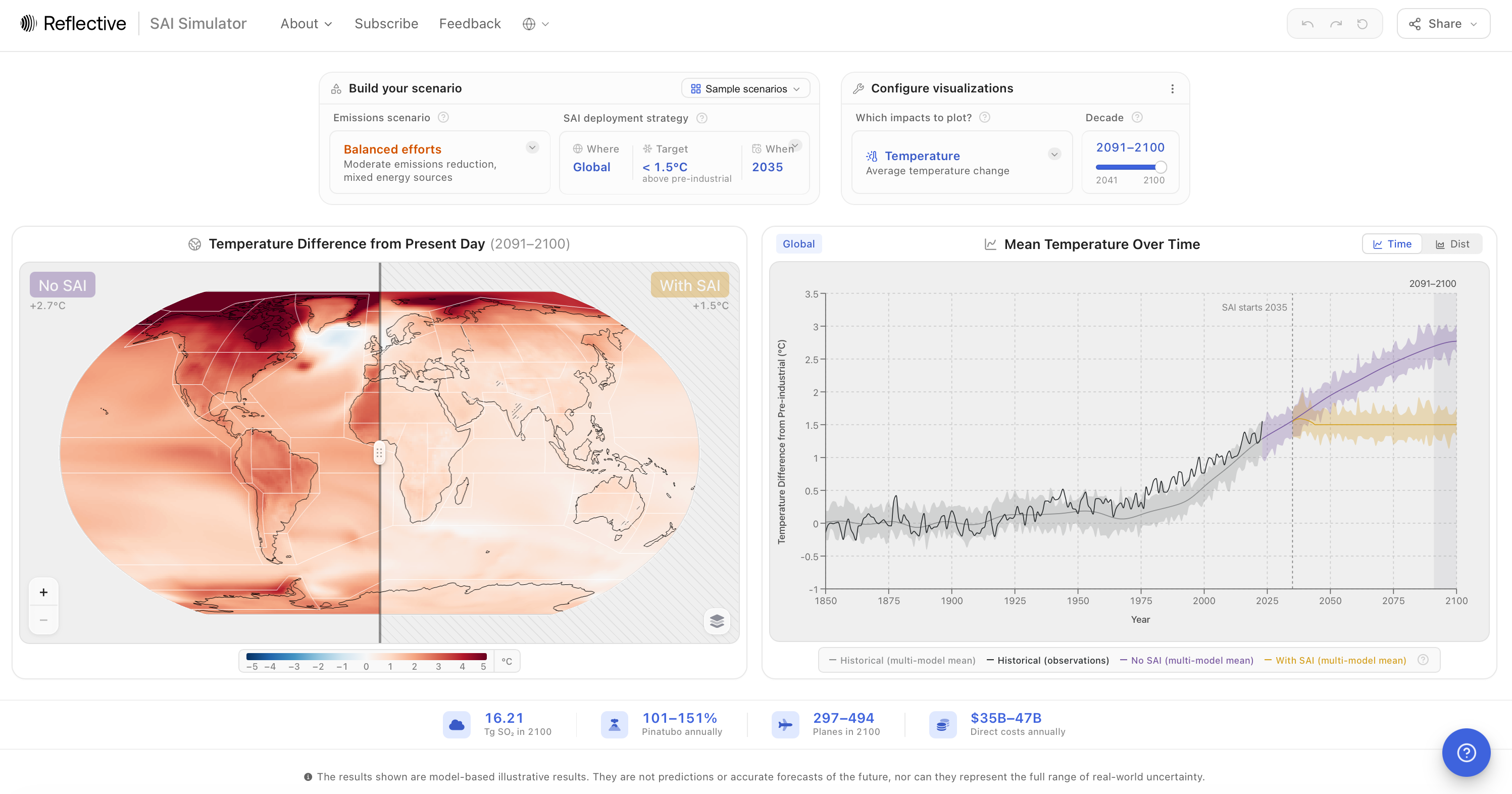
- Build your scenario (top left): the emissions scenario and the SAI deployment strategy, plus Sample scenarios.
- Configure visualizations (top right): which impact to show and for which decade.
- Map (middle left): the world with and without SAI, side by side.
- Chart (middle right): the selected impact over time, or its distribution in the selected decade.
- Deployment numbers (bottom): how much SO₂ would be injected, and rough estimates of aircraft and costs.
- Help (the ? button, bottom corner): an introduction to SAI, the guided tour, video walkthroughs and frequently asked questions.
Useful controls
Every setting is saved in the page address. Copy the link and anyone who opens it sees the same scenario, including a custom injection grid.
On a phone
On screens narrower than a tablet, the Simulator opens a mobile version. It offers a four-step guided setup ("Help me get started") or a scrolling overview of your scenario, the map, the chart and the deployment numbers. The Explore view shows the map and chart full screen. One feature is only available on desktop: editing injection values directly.
Step 1: Choose an emissions scenario
The emissions scenario sets how much the world warms without SAI. The Simulator uses the standard Shared Socioeconomic Pathways (SSPs) that climate scientists use to explore different futures. Our World in Data has a good introduction to them.
The default is SSP2-4.5, "Balanced efforts", a middle-of-the-road scenario that is close to current policies.
| Scenario | Name in the Simulator | Description | Approximate warming by 2081-2100, no SAI |
| SSP1-1.9 | Aggressive climate action | Rapid emissions cuts, global clean energy transition | 1.4°C |
| SSP1-2.6 | Strong climate action | Significant emissions reduction, clean energy adoption | 1.8°C |
| SSP4-3.4 | High inequality | Some climate action, uneven global progress | 2.2°C |
| SSP5-3.4 | Fossil fuels & CO₂ removal | High carbon use offset by removal technologies | 2.4°C |
| SSP2-4.5 | Balanced efforts | Moderate emissions reduction, mixed energy sources | 2.7°C |
| SSP4-6.0 | Inequality, minimal action | Limited climate measures, growing global disparity | 3.4°C |
| SSP3-Baseline | Geopolitical conflict | Minimal climate action, regional rivalries | 3.6°C |
| SSP5-Baseline | High fossil fuel use | Rapid growth, energy-intensive lifestyles | 4.4°C |
Warming is relative to pre-industrial times (1850–1900), based on the IPCC Sixth Assessment Report.
Step 2: Set the SAI deployment strategy
Click the SAI deployment strategy tile to set three things: where SAI is injected, how much SAI to do i.e. which target temperature to hold, and when research and deployment begin.
Where: the injection location
Where the particles are released affects where the cooling happens. The Simulator offers six options:
| Location | What it means |
| Global (default) | Injection at 15° and 30° north and south, with amounts adjusted each year to keep cooling even across the globe. This follows the strategy used in the ARISE climate model simulations. |
| Uniform | Equal injection at the equator and at 15°, 30° and 60° north and south. |
| Temperate zones | Injection over the mid-latitudes, at 30° north and south. |
| Polar | Injection only over the far north and south, at 60° north and south. |
| Polar, with backup | Focused on the poles, with extra injection across the mid-latitudes. |
| Northern Hemisphere only | Injection limited to the northern half of the planet. |
Locations other than Global are available for Temperature, Max and Min Temperature, Water Availability and Arctic Sea Ice.
Target: how much cooling
The target is the global average temperature, above pre-industrial levels, that SAI holds the world at. "< 1.5°C above pre-industrial" means SAI is used to keep global warming below 1.5 °C. A lower target means more cooling and more SO₂. The slider runs from 0.5 °C ("Aggressive cooling") to 2.5 °C ("Minimal cooling"); the default is 1.5 °C, in line with the Paris Agreement goal.
For every location, the Simulator works out how much SO₂ is needed each year to hold the target.
When: research and deployment
The timeline has two handles: when dedicated research and development (R&D) on SAI starts, and when deployment starts. Deployment can begin no earlier than five years after R&D starts, and no earlier than 2035. By default, R&D starts in 2030 and deployment in 2035.
If your target doesn't need SAI until later, for example because the emissions scenario stays below the target for a while, the Simulator moves the deployment year to the first year SAI is needed. Once deployment starts, SAI ramps up gradually over 10 years.
The rapid cooling warning
Some scenarios need the planet to cool faster than it is currently warming (about 0.23 °C per decade). When this happens, the chart shows a "⚠ Assumes rapid cooling: Potentially undesirable" label, and a ⚠ symbol appears next to the target. Cooling this quickly has not been shown to be achievable safely, and it could be harmful for some ecosystems. Starting earlier or choosing a higher target removes the warning.
Alternatively: Start from a sample scenario
Sample scenarios set the emissions scenario, deployment strategy and timeline in one click. Open them with Sample scenarios in the Build your scenario card. Each one is a starting point you can change.
| Sample scenario | Setup |
| Late deployment | SSP2-4.5, Global, below 1.5 °C, deployment from 2045 |
| Polar-only | SSP3-Baseline, injection at 60° north and south, deployment from 2035 |
| Ambitious climate policies | SSP1-2.6, Global, below 1.5 °C, deployment from 2035 |
| Shaving off the peak | SSP5-3.4, Global, below 2.0 °C, deployment from 2035 |
| Single actor, imbalanced deployment | SSP4-6.0, injection at 15° north only, up to 15 Tg per year, deployment from 2051 |
| Termination shock | SSP2-4.5, injection at all latitudes for four decades, stopped in 2081 |
Scenarios that use a custom injection grid (Polar-only, Single actor and Termination shock) are greyed out when the selected impact doesn't support custom injection.
Step 4 (optional): Edit injection values directly
For full control, open the SAI deployment strategy tile and choose Edit values directly. Instead of setting a target, you set exactly how much SO₂ is injected at each latitude in each decade. This option is available on desktop only.
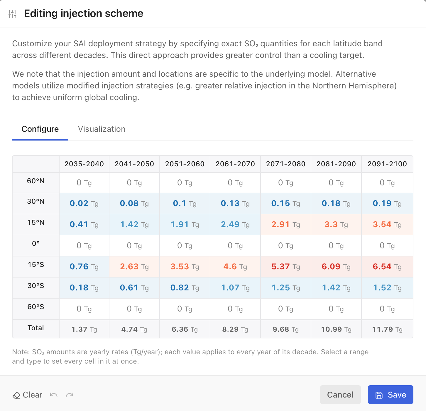
- The grid has seven latitude bands (60°N, 30°N, 15°N, 0°, 15°S, 30°S and 60°S) and seven periods (2035–2040, then each decade to 2091–2100). A Total row adds up the bands.
- Values are yearly rates in Tg of SO₂ per year. Each value applies to every year of its period. Select a range of cells and type a number to fill them all at once.
- Periods before research completes are locked, because deployment can't begin before then.
- Limits. Each cell can be between 0 and 150 Tg per year. If the total across all bands goes above 30 Tg per year, the Simulator warns you, because that is beyond the range the model can reasonably simulate. You can still save.
- The Visualization tab shows your schedule as a chart for each latitude band.
Save to apply the schedule. The strategy tile then shows "Custom scheme", with the peak injection rate, the number of active latitude bands and the years of injection. Reset returns to the default Global strategy.
Custom injection works for Temperature, Max and Min Temperature, Water Availability and Arctic Sea Ice. The climate response to custom injection is based on one climate model, CESM2-WACCM; treat the results as an indication of the pattern rather than a precise estimate.
Step 5: Choose what to show
Which impact?
Choose an impact under "Which impacts to plot?". Hover over the menu for a short description of each.
| Impact | What it shows | Unit |
| Temperature | Annual average air temperature near the surface. | °C |
| Max Temperature | The warmest temperature of the year. | °C |
| Min Temperature | The coldest temperature of the year. | °C |
| Extreme Heat Exposure | Person-days per year with average daily temperature above 40 °C. | million person-days |
| Heat Exposure | Person-days per year with average daily temperature above 35 °C. | million person-days |
| Freezing Exposure | Person-days per year with average daily temperature below 0 °C. | million person-days |
| Water Availability | Precipitation minus evaporation over land. Positive values mean more water available. | mm per day |
| Heavy Rain Exposure | Person-days per year with more than 20 mm of rain in a day. | million person-days |
| Rain Exposure | Person-days per year with more than 10 mm of rain in a day. | million person-days |
| Arctic Sea Ice Extent | Arctic sea ice in September, when it is at its smallest. | million km² |
Person-days combine how many people are exposed with how often. One person exposed for 10 days and 10 people exposed for one day both count as 10 person-days. The Simulator uses a fixed map of today's population.
Which decade?
Choose the decade shown on the map and in the distribution chart, from 2041–2050 to 2091–2100. The default is 2091–2100. Only decades after deployment starts are offered.
Visualization options
The ⋮ menu in the Configure visualizations card has three settings:
- Significance hatching (off by default): marks map areas where the change from present-day (1995–2014) levels is not statistically significant.
- Consistent scales: keeps the axes fixed, so you can compare scenarios and regions directly.
- Appearance: light, dark, or match your system.
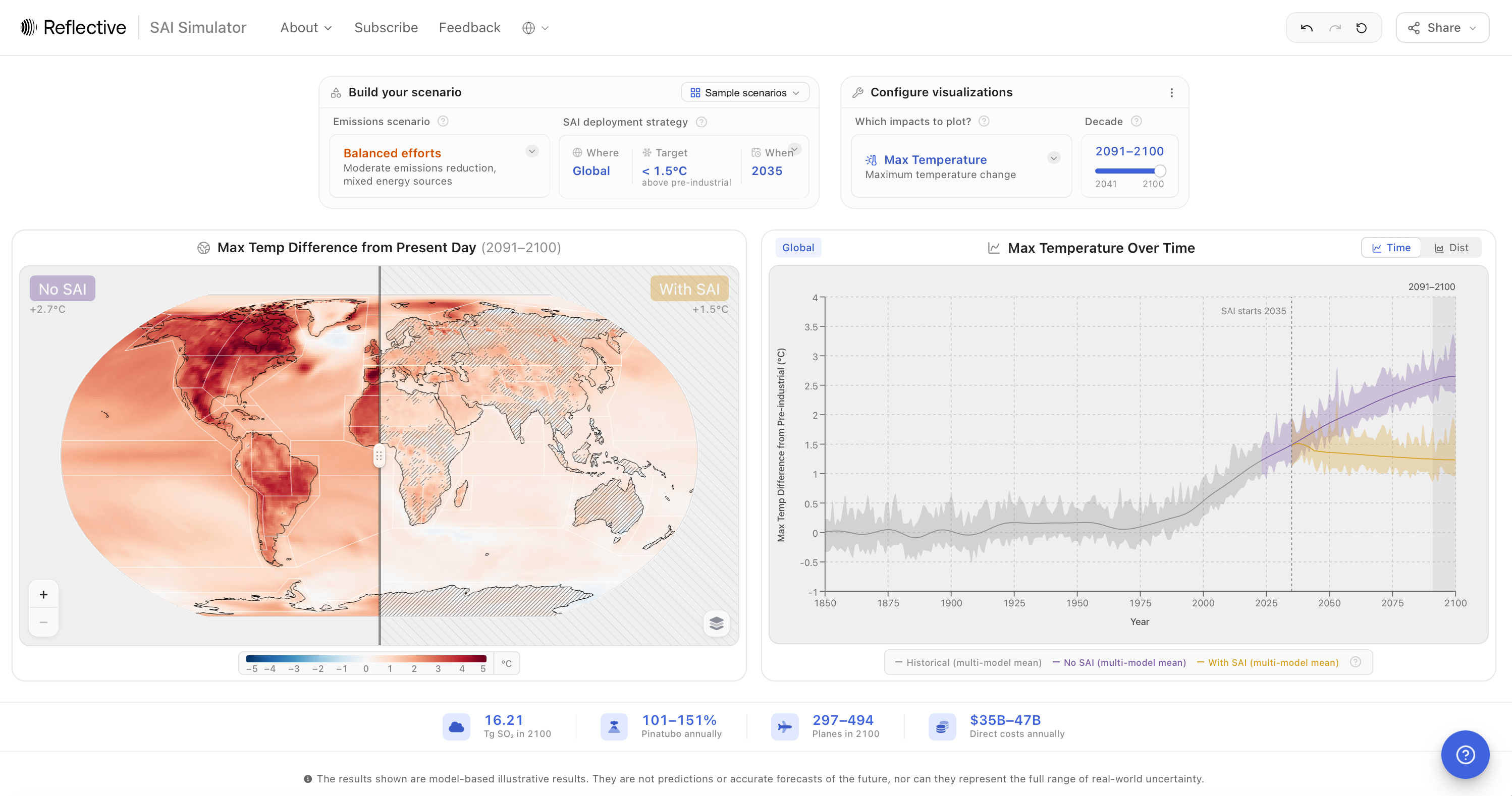
Reading the map
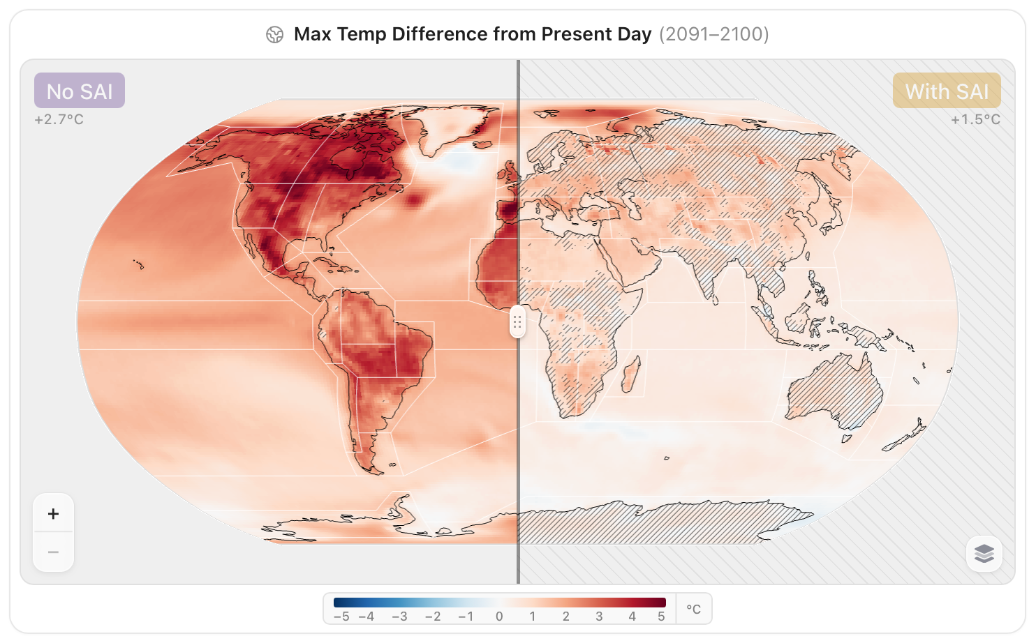
The map compares the world without SAI (left) and with SAI (right) for the selected decade. Drag the handle across the map to move between the two. The labels above each side give the global average temperature for that decade.
The map shows change from today's climate. Map values are relative to the present-day average (1995–2014), so they show how much warmer, wetter or drier a place would be compared with today. The line charts, by contrast, show change since pre-industrial times (1850–1900). The world was already about 0.6 °C warmer in 1995–2014 than in 1850–1900, so a 1.5 °C target appears as about +0.9 °C on the map.
- Regions. Click a region to show its results in the chart, and click it again (or Clear) to return to the global view. Choose a region set from the menu on the map: IPCC reference regions (58), continental regions (8), monsoon regions (6), major river basins (28) or small islands (9). Hovering a set previews its outlines.
- Significance hatching, when switched on, covers areas where the change is not statistically significant.
- Sea ice is shown on a map centred on the North Pole, as the fraction of ocean covered by ice. Regions are not available for sea ice.
- Latitude lines at 60°N to 60°S appear when a custom or latitude-specific injection is active, so you can see where SO₂ is injected.
- Use the + and − buttons, scrolling or pinching to zoom.
Reading the chart
The chart shows the selected impact for the whole world, or for the region you clicked. Switch between two views with Time and Dist.
Time: change over time
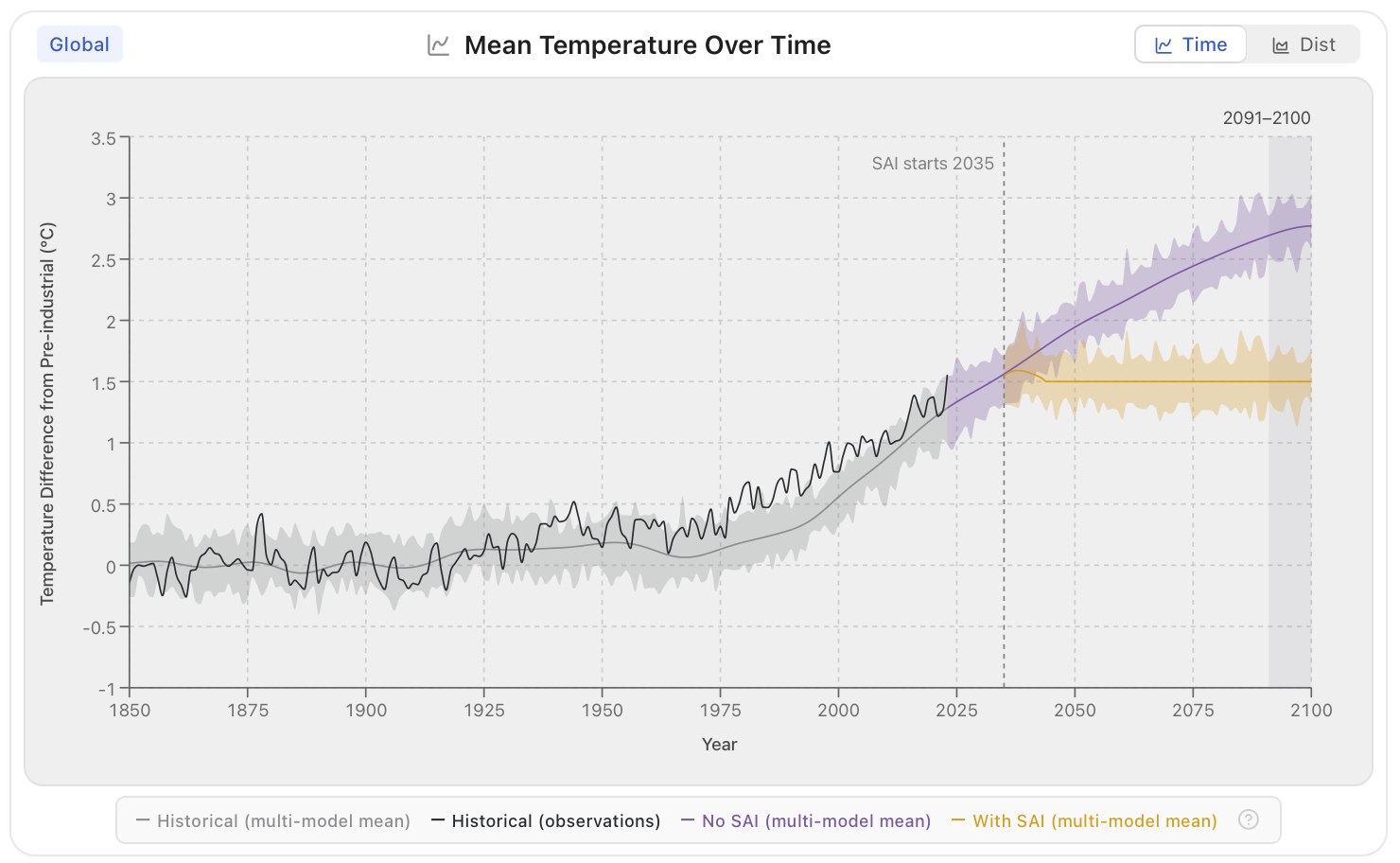
- Historical: the climate models' simulation of the past.
- Historical (obs.): observed temperature (1850–2024) and sea ice (1979–2025), shown for the global view.
- No SAI: the future under your emissions scenario.
- SAI: the same future with your SAI strategy.
All model lines are the average of the three climate models (except for customized injection strategies). A dashed line marks when SAI starts ("SAI starts 2035"), and the selected decade is highlighted. Values are relative to pre-industrial times (1850–1900).
The shading around each line shows the range of natural year-to-year climate variability: how much a single year could differ from the average because of the climate's own ups and downs. Hover over the chart to see the values for each year and the definition of the shading. The shading does not include disagreement between the climate models or other sources of uncertainty, so the total uncertainty is larger.
Dist: distribution in the selected decade
The distribution view shows how common each value is across the map grid in the selected decade, with and without SAI, compared with the historical period 1950–1959. Exposure and sea ice are shown as bar charts. Each grid cell counts equally, so areas near the poles, where grid cells are smaller, are over-represented compared with their actual area.
Deployment by the numbers
The cards below the map and chart summarise what your scenario would take. They update with the selected decade.
- Tg SO₂: the SO₂ injected into the stratosphere in the last year of the selected decade, in teragrams (millions of tonnes).
- Pinatubo annually: the decade's average yearly injection as a percentage of the SO₂ released by the 1991 eruption of Mount Pinatubo (about 10.4–15.5 Tg), which cooled the Earth by about 0.5 °C.
- Planes: the aircraft fleet needed in the last year of the decade, assuming each plane carries 15 tonnes per flight and flies 6–10 flights a day, all year.
- Direct costs annually: the yearly cost of deployment itself, based on the decade's average injection. It excludes indirect costs such as economic impacts or liability.
These are rough estimates; very little engineering work has been done on SAI delivery. Hover over each card for its sources.
Share, export and cite
Open the Share menu at the top right.
- Copy link copies a link to your exact scenario.
- Send link opens an email with the link and a short message.
- Generate citation formats a citation for the Simulator in APA, Harvard, MLA, Vancouver, Chicago or IEEE style, optionally with a link to your scenario.
- Download NetCDF downloads the results for the selected impact as a NetCDF file, a standard format for climate data that can be opened with tools such as Python (xarray), R or Panoply. Variables, years and latitude/longitude dimensions included.
Learn more
The ? button in the bottom corner opens the Help Center:
- What is SAI?: a four-step introduction to SAI, its potential benefits and risks.
- How to use the simulator: the guided tour.
- DEGREES walkthroughs: video walkthroughs of the Simulator by researchers from the DEGREES Initiative.
- Frequently asked questions: answers on aerosols, feasibility, risks and uncertainty.
In the About menu at the top you will also find this guide, the Model validation and Model comparison pages, and video tours.
Feedback
We want to hear how you use the Simulator and what would make it more useful. Use the feedback form, linked as Feedback at the top of the Simulator.